Week 3 Lab: Data Processing (Part 1)

This lab gives you hands-on practice with the data processing decisions from lecture using engineered versions of the corn yield and drought datasets you collected last week. In each section, you will work with modified data that introduces realistic challenges: missing values, untidy structure, and temporal aggregation decisions.

Learning Objectives

By the end of the lab, you will be able to:

Quantify and visualize missing data patterns
Distinguish between types of missingness and apply appropriate handling strategies
Reshape untidy data into tidy form using pivot_longer() and pivot_wider()
Aggregate time-series data to match your research question
Document your data processing choices
Learn the basics of the dplyr and tidyr packages for data manipulation

Preliminaries

Create a folder called lab_03 and navigate there in RStudio.
Create a new R script called lab_03.R in your lab_03 folder.
Write a brief comment at the top describing the purpose of the script and your name.
Load required libraries at the top:

library(tidyverse)

Lab Notebook

Open up a word processing document (e.g., Google Doc, Word, or plain text) to serve as your lab notebook. Use this to respond to questions, document decisions, and reflect on the process. You should also comment your R script thoroughly to explain your code and rationale for each step.

Section 1: Missing Data

Context

Real datasets often contain missing values (R represents missing data as NA). But “missing” can mean different things:

MAR (Missing at Random): Missingness is unrelated to any variables
MNAR (Missing at Random): Missingness depends on observed or unobserved data (e.g., low-yield years less likely to be reported)

Your processing choice—deletion, imputation, or flagging—depends on understanding why data are missing. How to deal with missing data is a whole area of study. We will investigate the consequences of missing data, but not implement any solutions because it requires analysis we have not yet covered. There are many resources online.

Data

The file corn_yield_missing.csv contains engineered missingness:

Random MCAR: ~5% of yield values randomly set to NA
Informative MAR: Systematic missing values for certain states and years (mimicking reporting thresholds)

The function read_csv() can read data from a local file path or a URL. You can download the file from the course repository and save it in your lab_03 folder, or read it directly from the url.

Task

Optional (Excel): Quantify missingness in Excel

If you want to do a quick check in MS Excel before working in R, use the steps below. In the dataset, the yield variable is Value (and there are two engineered versions, Value_mar and Value_mnar).

Open the CSV in Excel.
Turn on Filters (Data → Filter).
In the Value column filter drop‑down, check NA to see missing rows.
Count how many rows are NA in Value:

In a blank cell, enter =COUNTIF([Value], "NA").

Count total rows (excluding the header):

Use =COUNTA([Value]).

Compute the percent missing:

=COUNTIF([Value], "NA") / COUNTA([Value]).

You can repeat the same steps for Value_mar and Value_mnar to compare the three missingness patterns.

Quantify missingness in R

Load the data into R using read_csv(), then use glimpse() to inspect the structure and data types.

# Read the data with missing values
corn_missing <- read_csv("https://jbayham.github.io/arec-330/modules/03_data_processing/includes/corn_yield_missing.csv")

# Inspect the structure
glimpse(corn_missing)

Let’s begin by reaquinting ourselves with the data. The corn yield data contains many columns that we won’t need, so lets subset the columns to focus on what we do need. Let’s use the select() function to keep only the columns that are relevant for our analysis. We will keep the following columns:

state_alpha: State abbreviation (e.g., “IA” for Iowa)
commodity_desc: Description of the commodity (e.g., “CORN”)
year: Year of the observation
Value: The original yield value (with engineered missingness)
Value_mar: The version of yield with MAR missingness
Value_mnar: The version of yield with MNAR missingness

corn_missing_sub <- select(corn_missing, state_alpha, commodity_desc, year, Value, Value_mar, Value_mnar)

Count Missing Values

Now we can focus on the columns that are relevant for our analysis. The Value columns is complete. Let’s quantify the missingness in the columns Value_mar and Value_mnar to understand the extent of missing data we are dealing with. We can use the is.na() function to identify missing values and then summarize the total count and proportion of missingness.

#Apply the is.na() function to the Value_mar column to identify missing values
is.na(corn_missing_sub$Value_mar)

That generates a logical vector where TRUE indicates a missing value and FALSE indicates a non-missing value. To quantify the total number of missing values, we can use the sum() function, which will count the number of TRUE values in the logical vector. To calculate the proportion of missing values, we can take the sum of missing values and divide it by the total number of observations (rows) in the dataset..

# Quantify total missingness
sum(is.na(corn_missing_sub$Value_mar))
sum(is.na(corn_missing_sub$Value_mar))/nrow(corn_missing_sub)  # proportion missing
#or 
mean(is.na(corn_missing_sub$Value_mar))  # proportion missing

Do the same for the column Value_mnar on your own

Question 1: Which column has more missing values, Value_mar or Value_mnar? What does this suggest about the nature of the missingness in each column? Answer in your notebook.

Explore Missingness by State and Year

Now we want to quantify missingness by state and year to see if there are patterns. We can use the group_by() and summarize() functions to calculate the number of missing values for each state and year combination. The function summarize() will allow us to create a new summary dataset that contains the count of missing values for each group. The function group_by() will group the data by the specified columns (in this case, state_alpha and year) so that the summary statistics are calculated for each unique combination of state and year.

# Group by state, then summarize missingness
corn_missing_sub_grp <- group_by(corn_missing_sub, state_alpha)

corn_missing_summary <- summarize(corn_missing_sub_grp,
                                  n_missing_mar = sum(is.na(Value_mar)),
                                  n_missing_mnar = sum(is.na(Value_mnar)),
                                  total_obs = n(),
                                  prop_missing_mar = n_missing_mar / total_obs,
                                  prop_missing_mnar = n_missing_mnar / total_obs)

Do the same for grouping by year on your own.

Question 2: Are there certain states or years that have higher proportions of missing data? What might be some reasons for this pattern? Answer in your notebook.

Consequences of Missing Data

Finally, we want to understand the consequences of missing data for our analysis. Let’s calculate the mean yield for each of the variables (Value, Value_mar, and Value_mnar). This will help us understand how much bias might be introduced by missing data. We will use summarize() again to calculate the mean yield for each column, while ignoring the missing values using the argument na.rm = TRUE.

# Calculate mean yield for each column
yield_summary <- summarize(corn_missing_sub,
                          mean_value = mean(Value, na.rm = TRUE),
                          mean_value_mar = mean(Value_mar, na.rm = TRUE),
                          mean_value_mnar = mean(Value_mnar, na.rm = TRUE))

Question 3: How do the mean yields compare across the three columns? What does this suggest about the potential bias introduced by missing data? Answer in your notebook.

Section 2: Reshaping Untidy Data

Context

“Tidy data” follows three rules:

Each variable is a column
Each observation is a row
Each type of observational unit is a separate table

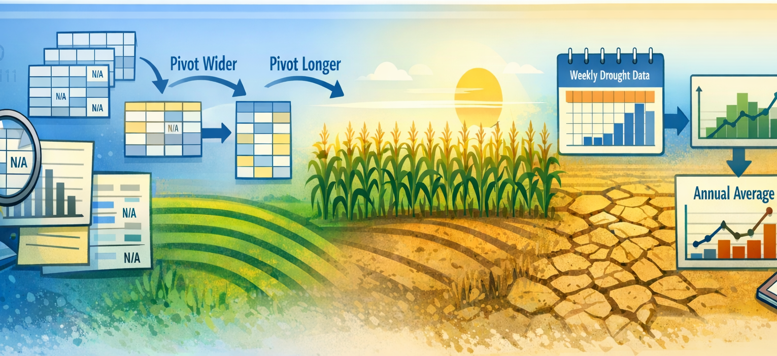
Real data rarely arrive in tidy form. The pivot_longer() and pivot_wider() functions let you reshape data flexibly.

Data

The corn yield data are already in a tidy format, but let’s pretend they are not.

Tasks

Task 2.1: Load and Inspect Untidy Data

corn_wide <- read_csv("https://jbayham.github.io/arec-330/modules/03_data_processing/includes/corn_wide.csv")

glimpse(corn_wide)

# Look at the first few rows to understand the structure
head(corn_wide)

Question 4: What makes this data “untidy”? Describe how the structure differs from the tidy format. Answer in your notebook.

In R, calculate the average corn yield for each state across all years using the original wide format. Make sure to include this in your script.

Task 2.2: Reshape to Tidy Format

The tidyverse provides a useful function for reshaping data called, pivot_longer(). This function takes multiple columns that represent different categories (e.g., years) and pivots them into a longer format where there is a single column for the category (e.g., “year”) and a single column for the values (e.g., “yield”). The arguments to pivot_longer() specify which columns to pivot, the name of the new category column, and the name of the new value column.

corn_tidy <- pivot_longer(corn_wide,
                         cols = starts_with("year_"),  # columns for each year
                         names_to = "year",  # new column for year
                         names_prefix = "year_",  # remove "year_" prefix from year values
                         values_to = "yield")  # new column for yield


# Inspect the result
glimpse(corn_tidy)
head(corn_tidy, 10)

Question 5: How has the structure of the data changed after pivoting? How many rows do you have now? What are the new variables created, and how do they relate to the original columns? What is the data type of the year variable? Is that desirable? Answer in your notebook.

Now calculate the average corn yield for each state across all years using the tidy format. Compare your results to the average yields you calculated in the previous task using the wide format. Are they the same? Which method was easier to use and why? Make sure to include this in your script.

Section 3: Temporal Aggregation

Context

Your corn yield data are annual (one value per state per year), but your drought data are weekly (52+ values per state per year). Before merging, you must aggregate drought data to match.

But how you aggregate depends on your question:

Simple annual average: best for year-over-year comparisons
Growing season window: focuses on when drought matters biologically
Critical period: captures timing of drought stress relative to crop development
Cumulative measures: emphasizes total exposure

We will calculate a single simple drought metric for each state-year for now. In future labs, we will explore more complex temporal features and how they affect the drought-yield relationship.

Data

We will will now transition to the drought dataset, which contains weekly observations of drought severity for each state from 2000 to 2025.

drought_dat <- read_csv("https://jbayham.github.io/arec-330/modules/03_data_processing/includes/dm_state_2000-2025.csv")

glimpse(drought_dat)

Tasks

Task 3.1: Calculate the Drought Severity Composite Index (DSCI)

The drought dataset contains the area of each state in different drought categories (None, D0, D1, D2, D3, D4) for each week. To create a single drought severity metric, we will calculate the Drought Severity Composite Index (DSCI), which is a weighted average of the area in each drought category. The DSCI gives us a single value that represents the overall drought severity for each state-week observation.¹ The formula is: \[DSCI = \frac{0 \times \text{Area}_{None} + 1 \times \text{Area}_{D0} + 2 \times \text{Area}_{D1} + 3 \times \text{Area}_{D2} + 4 \times \text{Area}_{D3} + 5 \times \text{Area}_{D4}}{\text{Total Area}}\]

In R, we will use the mutate() function (from dplyr) to create a new variable dsci that calculates the DSCI for each state-week observation. We will also calculate the total_area for each state-week to use in the denominator of the DSCI formula.

# Calculate DSCI as a weighted sum of severity levels
drought_weekly <- drought_dat %>%
  mutate(
    total_area = None + D0 + D1 + D2 + D3 + D4,
    dsci = (0 * None + 1 * D0 + 2 * D1 + 3 * D2 + 4 * D3 + 5 * D4)/total_area
  )

Question 6: Explain to a non-technical audience what the DSCI represents and how it is calculated. Why might this be a useful metric for summarizing drought severity? Answer in your notebook.

Task 3.2: Strategy A - Simple Annual Average

Now we need to aggregate the weekly drought data to an annual level. The simplest approach is to calculate the average DSCI for each state-year. This gives us a single drought severity value for each state and year, which we can then merge with the corn yield data. We will use the group_by() and summarize() functions to perform this aggregation. We will group the data by StateAbbreviation and year, then calculate the mean DSCI for each group.

First, we need to extract the year from the ValidStart date column. We can use the year() function from the lubridate package to do this. Then we will group by state and year, and calculate the mean DSCI.

We also want to introduce the pipe operator (%>%) to chain our operations together in a clear and readable way. The pipe allows us to take the output of one function and pass it directly into the next function without needing to create intermediate objects.

drought_annual <- drought_weekly %>%
  mutate(year = year(ValidStart)) %>%
  group_by(StateAbbreviation, year) %>%
  summarize(
    mean_dsci = mean(dsci, na.rm = TRUE),
    .groups = "drop"
  )

head(drought_annual)

Question 7: What does the mean_dsci variable represent in the drought_annual dataset? How does this aggregation help us prepare the drought data for merging with the corn yield data? What are some potential limitations of using a simple annual average to summarize drought severity? Answer in your notebook.

Deliverables

Submit the following on Canvas:

Organize your code and make sure it runs without errors. Then generate a log file called lab_03.log using the sink-source-sink pattern from previous labs. The log file should include all the code you wrote for this lab, along with comments explaining each step.
Notebook responses: Compile your answers to the questions in a single document (e.g., Google Doc, Word, or plain text). Make sure to clearly label each question and provide thoughtful, detailed responses based on your analysis.

Footnotes

https://droughtmonitor.unl.edu/About/AbouttheData/DSCI.aspx ↩︎